Trajectories Module

The objective of the trajectory module is to ease the handling of multiple risk assessment at different point in time, and enable interpolation in time.

Quickstart example

In the following example we use the DEMO data to showcase the basic workflow to use this module.

As usual, a thourough read of this tutorial is highly recommended!

from climada.hazard import Hazard
from climada.util import HAZ_DEMO_H5
from climada.entity import Entity
from climada.util.constants import ENT_DEMO_FUTURE, ENT_DEMO_TODAY
from climada.trajectories.snapshot import Snapshot
from climada.entity import ImpactFuncSet, ImpfTropCyclone
from climada.trajectories import StaticRiskTrajectory, InterpolatedRiskTrajectory
import warnings

warnings.simplefilter("ignore")

# Load exposure
exp_present = Entity.from_excel(ENT_DEMO_TODAY).exposures
exp_future = Entity.from_excel(ENT_DEMO_FUTURE).exposures

# Load Hazard
haz_present = Hazard.from_hdf5(HAZ_DEMO_H5)
haz_future = Hazard.from_hdf5(HAZ_DEMO_H5)
haz_future.frequency *= 1.2

# Load impact function set
impf_tc_present = ImpfTropCyclone.from_emanuel_usa()
impf_tc_future = ImpfTropCyclone.from_emanuel_usa(v_half=70.0)
impf_set_present = ImpactFuncSet([impf_tc_present])
impf_set_future = ImpactFuncSet([impf_tc_future])

# Create the snapshots
snap1 = Snapshot(
    exposure=exp_present, hazard=haz_present, impfset=impf_set_present, date="2018"
)

snap2 = Snapshot(
    exposure=exp_future, hazard=haz_future, impfset=impf_set_future, date="2050"
)

# Create the trajectory
interpolated_risk_traj = InterpolatedRiskTrajectory([snap1, snap2])

# Observe the results
display(interpolated_risk_traj.per_date_risk_metrics())

interpolated_risk_traj.plot_waterfall()
interpolated_risk_traj.plot_time_waterfall()

2026-03-27 14:39:25,551 - climada.hazard.io - INFO - Reading /home/sjuhel/climada/demo/data/tc_fl_1990_2004.h5
2026-03-27 14:39:25,587 - climada.hazard.io - INFO - Reading /home/sjuhel/climada/demo/data/tc_fl_1990_2004.h5
2026-03-27 14:39:25,752 - climada.trajectories.calc_risk_metrics - WARNING - No group id defined in at least one of the Exposures object. Per group aai will be empty.

	date	group	measure	metric	unit	risk
0	2018	All	no_measure	aai	USD	2.888955e+08
1	2019	All	no_measure	aai	USD	3.029192e+08
2	2020	All	no_measure	aai	USD	3.172858e+08
3	2021	All	no_measure	aai	USD	3.319988e+08
4	2022	All	no_measure	aai	USD	3.470618e+08
...	...	...	...	...	...	...
127	2046	All	no_measure	rp_100	USD	3.669278e+10
128	2047	All	no_measure	rp_100	USD	3.773739e+10
129	2048	All	no_measure	rp_100	USD	3.879833e+10
130	2049	All	no_measure	rp_100	USD	3.987570e+10
131	2050	All	no_measure	rp_100	USD	4.096960e+10

132 rows × 6 columns

(<Figure size 1200x600 with 1 Axes>,
 <Axes: title={'center': 'Contributions to change in risk between 2018-01-01 00:00:00 and 2050-01-01 00:00:00 (Average)'}, ylabel='Deviation from base risk'>)

Important disclaimers

Interpolation of risk can be… risky

One purpose of this module is to improve the evaluation of risk in between two “known” points in time.

This part relies on interpolation (linear by default) of impacts and risk metrics in between the different specified points, which may lead to incoherent results in cases where this simplification drifts too far from reality.

For instance if you are using different historical events as you points in time, a static comparison of the different risk estimates may be interesting, but interpolating in between makes very little sense.

Memory and computation requirements

This module adds a new dimension (time) to the risk, as such, it multiplies the memory and computation requirement along that dimension (although we avoid running a full-fledge impact computation for each “interpolated” point, we still have to define an impact matrix for each of those).

This can of course (very) quickly increase the memory and computation requirements for bigger data. We encourage you to first try on small examples before running big computations.

Using the trajectories module

The fundamental idea behing the trajectories module is to enable a better assessment of the evolution of risk over time, both by facilitating point by point comparison, and the “evolution” or risk.

This module aims at facilitating answering questions such as:

• How does future hazards (probabilistic event set), exposure and vulnerability change impacts with respect to present?

• How would the impacts compare if a past event were to happen again with present / future exposure?

• How will risk evolve in the future under different assumptions on the evolution of hazard, exposure, vulnerability and discount rate?

• etc.

To achieve this, this module introduces two concepts:

• Snapshots of risk, a fixed representation of risk (via its three components Exposure, Hazard and Vulnerability) for a given date. This concept is intended to be generic, as such the given date can be something else than a year, a month or a day for instance, but keep in mind that we will not check that the data you provide makes sense for it!

• Trajectories of risk, a collection of snapshots,for which risk metrics can be computed and regrouped to ease their evaluation.

Snapshot: A snapshot of risk at a specific year

We use Snapshot objects to define a point in time for risk. This object acts as a wrapper of the classic risk framework composed of Exposure, Hazard and Vulnerability. As such it is defined for a specific date (usually a year), and contains an Exposures, a Hazard, and an ImpactFuncSet object.

Instantiating such a Snapshot is done simply with:

snap = Snapshot(
            exposure=your_exposure,
            hazard=your_hazard,
            impfset=your_impfset,
            date=your_date
            )

Note that to avoid any ambiguity, you need to write explicitly exposure=your_exposure.

Think of Snapshot as a representation of risk at, or around, a specific date. Your hazard should be a probabilistic set of events that are representative for the designated date.

To be consistent with the intuitive idea of a snapshot, by default Snapshot objects make a “deep copy” of the risk triplet and are immutable. This means that they do not change once created (notably even if you change one of the component, e.g. the Hazard object, outside of the Snapshot). If you want a Snapshot with a different Hazard, you need to create a new one.

In that spirit, you cannot directly instantiate a Snapshot with an adaptation measure. To include adaptation, you need to first create the snapshot without adaptation, and then use apply_measure(), which will return a new Snapshot, with the changed (Exposure, Hazard, ImpactFuncSet) according to the given measure.

You can supply a measure object to Snapshot(<...>, measure=measure), but it will not be applied to the triplet (Exposure, Hazard, ImpactFuncSet) and assume the triplet already include the change. Only advanced users with a good understanding of what they are doing should supply a measure parameter directly to the Snapshot constructor, else, stick to the apply_measure() method.

Below is an concrete example of how to create a Snapshot using data from the data API for tropical cyclones in Haiti:

from climada.util.api_client import Client
from climada.entity import ImpactFuncSet, ImpfTropCyclone
from climada.trajectories.snapshot import Snapshot

client = Client()

exp_present = client.get_litpop(country="Haiti")

haz_present = client.get_hazard(
    "tropical_cyclone",
    properties={
        "country_name": "Haiti",
        "climate_scenario": "historical",
        "nb_synth_tracks": "10",
    },
)

impf_set = ImpactFuncSet([ImpfTropCyclone.from_emanuel_usa()])
exp_present.gdf.rename(columns={"impf_": "impf_TC"}, inplace=True)
exp_present.gdf["impf_TC"] = 1

snap1 = Snapshot(
    exposure=exp_present, hazard=haz_present, impfset=impf_set, date="2018"
)

2026-03-27 14:39:27,625 - climada.entity.exposures.base - INFO - Reading /home/sjuhel/climada/data/exposures/litpop/LitPop_150arcsec_HTI/v3/LitPop_150arcsec_HTI.hdf5
2026-03-27 14:39:32,846 - climada.hazard.io - INFO - Reading /home/sjuhel/climada/data/hazard/tropical_cyclone/tropical_cyclone_10synth_tracks_150arcsec_HTI_1980_2020/v2/tropical_cyclone_10synth_tracks_150arcsec_HTI_1980_2020.hdf5

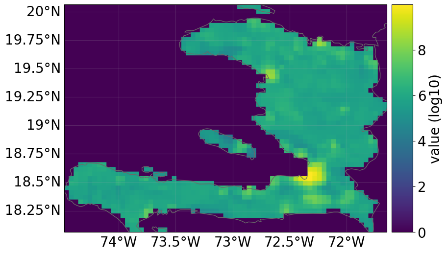
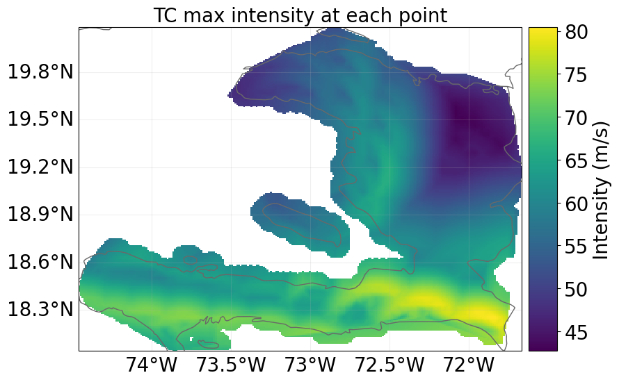
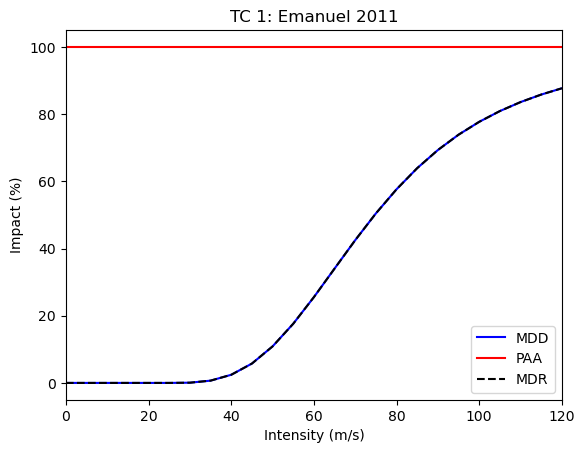
All risk dimensions are freely accessible from the snapshot:

snap1.exposure.plot_raster()
snap1.hazard.plot_intensity(0)
snap1.impfset.plot()

2026-03-27 14:39:32,894 - climada.util.coordinates - INFO - Raster from resolution 0.04166665999999708 to 0.04166665999999708.

<Axes: title={'center': 'TC 1: Emanuel 2011'}, xlabel='Intensity (m/s)', ylabel='Impact (%)'>

Evaluating risk from multiple snapshots using trajectories

Trajectories facilitate the evaluation of risk of multiple snapshot. The module implements two kinds of trajectories:

• StaticRiskTrajectory: which estimate the risk at each snaphot only, and regroups the results nicely.

• InterpolatedRiskTrajectory: which also includes the evolution of risk in between the snapshots using interpolation.

So first, let us define Snapshot for a future point in time. We will increase the value of the exposure following a certain growth rate, and use future tropical cyclone data for the hazard, we will also change the vulnerability to be slightly lower in the future:

import copy

future_year = 2040
exp_future = copy.deepcopy(exp_present)
exp_future.ref_year = future_year
n_years = exp_future.ref_year - exp_present.ref_year + 1
growth_rate = 1.02
growth = growth_rate**n_years
exp_future.gdf["value"] = exp_future.gdf["value"] * growth

haz_future = client.get_hazard(
    "tropical_cyclone",
    properties={
        "country_name": "Haiti",
        "climate_scenario": "rcp60",
        "ref_year": str(future_year),
        "nb_synth_tracks": "10",
    },
)

impf_set = ImpactFuncSet(
    [
        ImpfTropCyclone.from_emanuel_usa(v_half=78.0),
    ]
)
exp_future.gdf.rename(columns={"impf_": "impf_TC"}, inplace=True)
exp_future.gdf["impf_TC"] = 1
snap2 = Snapshot(
    exposure=exp_future, hazard=haz_future, impfset=impf_set, date=str(future_year)
)

### Now we can define a list of two snapshots, present and future:
snapcol = [snap1, snap2]

2026-03-27 14:39:40,926 - climada.hazard.io - INFO - Reading /home/sjuhel/climada/data/hazard/tropical_cyclone/tropical_cyclone_10synth_tracks_150arcsec_rcp60_HTI_2040/v2/tropical_cyclone_10synth_tracks_150arcsec_rcp60_HTI_2040.hdf5

Based on such a list of snapshots, we can then evaluate a risk trajectory using a StaticRiskTrajectory or a InterpolatedRiskTrajectory object.

from climada.trajectories import StaticRiskTrajectory, InterpolatedRiskTrajectory

static_risk_traj = StaticRiskTrajectory(snapcol)
interpolated_risk_traj = InterpolatedRiskTrajectory(snapcol)

Tidy format

We use the “tidy” format to output most of the results.

A tidy data format is a standardized way to structure datasets, making them easier to analyze and visualize. It’s based on three main principles:

1. Each variable forms a column.

2. Each observation forms a row.

3. Each type of observational unit forms a table.

Example:

group	date	metric	risk
All	2018-01-01	aai	\(1.840432 \times 10^{8}\)
All	2040-01-01	aai	\(6.946753 \times 10^{8}\)
All	2018-01-01	rp_20	\(1.420589 \times 10^{8}\)

In this example, every descriptive quality (variable) of the risk evaluation is placed in its own column:

• group: The exposure subgroup for the risk evalution point.

• date: The date for the risk evalution point.

• metric: The specific risk measure (e.g., ‘aai’, ‘rp_20’, ‘rp_100’).

• unit: The unit of the risk evaluation.

• risk: The actual value being measured.

Each row represents a single, complete observation. For example, the very first row is a measurement of the ‘aai’ metric for group ‘All’ on ‘2018-01-01’, with the resulting risk value of \(1.840432 \times 10^{8}\) USD.

Static and Interpolated trajectories

StaticRiskTrajectory will compute and hold risk metrics for all the given snapshots without interpolation:

static_risk_traj.per_date_risk_metrics()

2026-03-27 14:39:41,093 - climada.trajectories.calc_risk_metrics - WARNING - No group id defined in the Exposures object. Per group aai will be empty.

	date	group	measure	metric	unit	risk
0	2018-01-01	All	no_measure	aai	USD	1.840432e+08
1	2040-01-01	All	no_measure	aai	USD	2.749295e+08
2	2018-01-01	All	no_measure	rp_20	USD	1.420589e+08
3	2040-01-01	All	no_measure	rp_20	USD	2.357976e+08
4	2018-01-01	All	no_measure	rp_50	USD	3.059112e+09
5	2040-01-01	All	no_measure	rp_50	USD	4.580720e+09
6	2018-01-01	All	no_measure	rp_100	USD	5.719050e+09
7	2040-01-01	All	no_measure	rp_100	USD	8.477125e+09

The InterpolatedRiskTrajectory object goes further and computes the metrics for all the dates between the different snapshots in the given collection for a given time resolution (one year by default). In this example, from the snapshot in 2018 to the one in 2040.

Note that this can require a bit of computation and memory, especially for large regions or extended range of time with high time resolution. Also note, that most computations are only run and stored when needed, not at instantiation.

From this object you can access different risk metrics:

• Average Annual Impact (aai) both for all exposure points (group == “All”) and specific groups of exposure points (defined by a “group_id” in the exposure).

• Estimated impact for different return periods (20, 50 and 100 by default)

Both as average over the whole period:

interpolated_risk_traj.per_period_risk_metrics()

2026-03-27 14:39:42,146 - climada.trajectories.calc_risk_metrics - WARNING - No group id defined in at least one of the Exposures object. Per group aai will be empty.

	period	group	measure	metric	unit	risk
0	2018 to 2040	All	no_measure	aai	USD	2.309016e+08
1	2018 to 2040	All	no_measure	rp_100	USD	7.148372e+09
2	2018 to 2040	All	no_measure	rp_20	USD	1.896739e+08
3	2018 to 2040	All	no_measure	rp_50	USD	3.847129e+09

Or on a per-date basis:

interpolated_risk_traj.per_date_risk_metrics()

2026-03-27 14:39:42,191 - climada.trajectories.calc_risk_metrics - WARNING - No group id defined in at least one of the Exposures object. Per group aai will be empty.

	date	group	measure	metric	unit	risk
0	2018	All	no_measure	aai	USD	1.840432e+08
1	2019	All	no_measure	aai	USD	1.885312e+08
2	2020	All	no_measure	aai	USD	1.929908e+08
3	2021	All	no_measure	aai	USD	1.974211e+08
4	2022	All	no_measure	aai	USD	2.018214e+08
...	...	...	...	...	...	...
87	2036	All	no_measure	rp_100	USD	8.025179e+09
88	2037	All	no_measure	rp_100	USD	8.140512e+09
89	2038	All	no_measure	rp_100	USD	8.254300e+09
90	2039	All	no_measure	rp_100	USD	8.366514e+09
91	2040	All	no_measure	rp_100	USD	8.477125e+09

92 rows × 6 columns

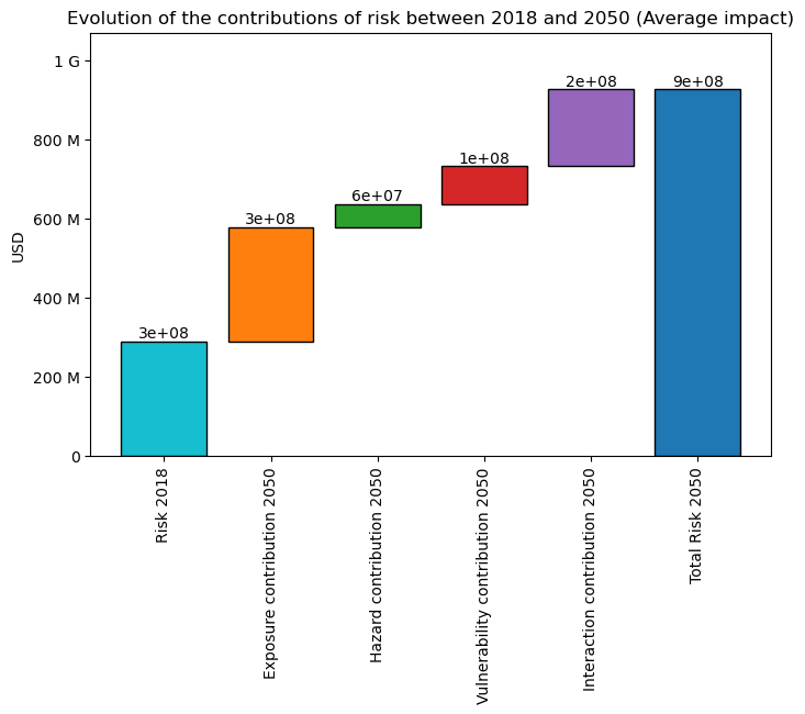
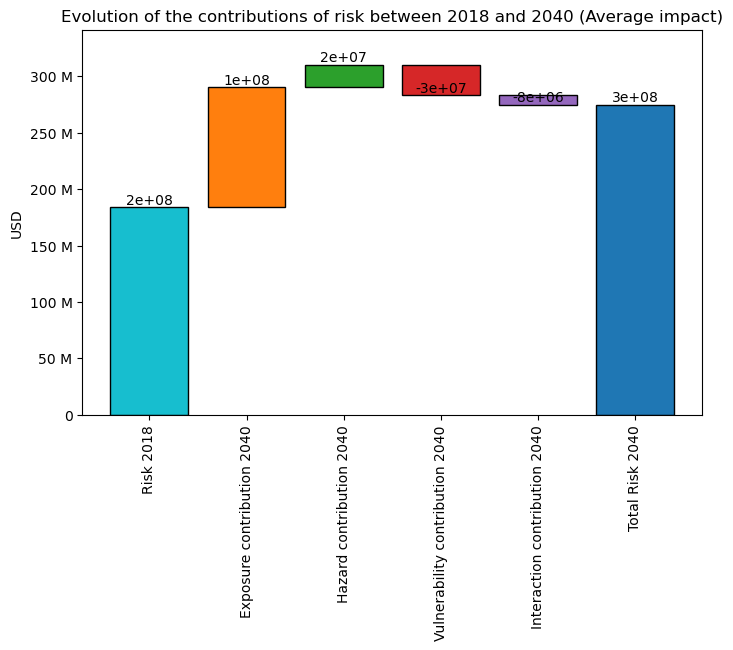
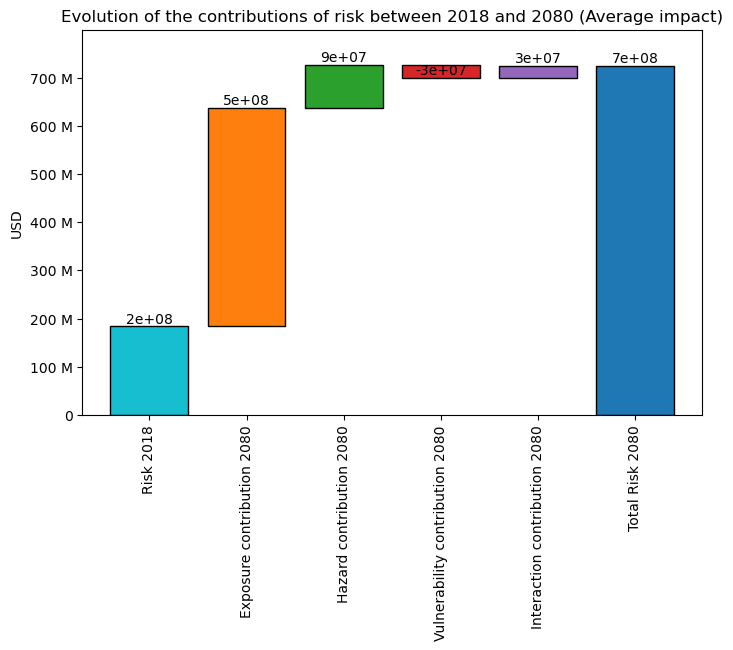
You can also plot the “contribution” or “components” of the change in risk (Average ) via a waterfall graph:

• The ‘base risk’, i.e., the risk without change in hazard or exposure, compared to trajectory’s earliest date.

• The ‘exposure contribution’, i.e., the additional risks due to change in exposure (only)

• The ‘hazard contribution’, i.e., the additional risks due to change in hazard (only)

• The ‘vulnerability contribution’, i.e., the additional risks due to change in vulnerability (only)

• The ‘interaction contribution’, i.e., the additional risks due to the interaction term (between exposure, hazard and vulnerability)

interpolated_risk_traj.plot_waterfall()

<Axes: title={'center': 'Evolution of the contributions of risk between 2018 and 2040 (Average impact)'}, ylabel='USD'>

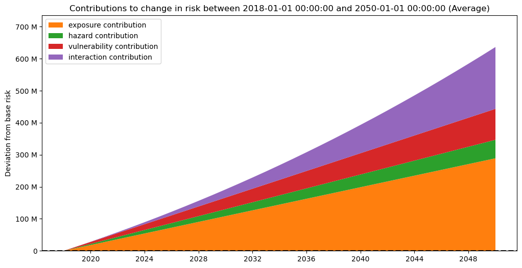
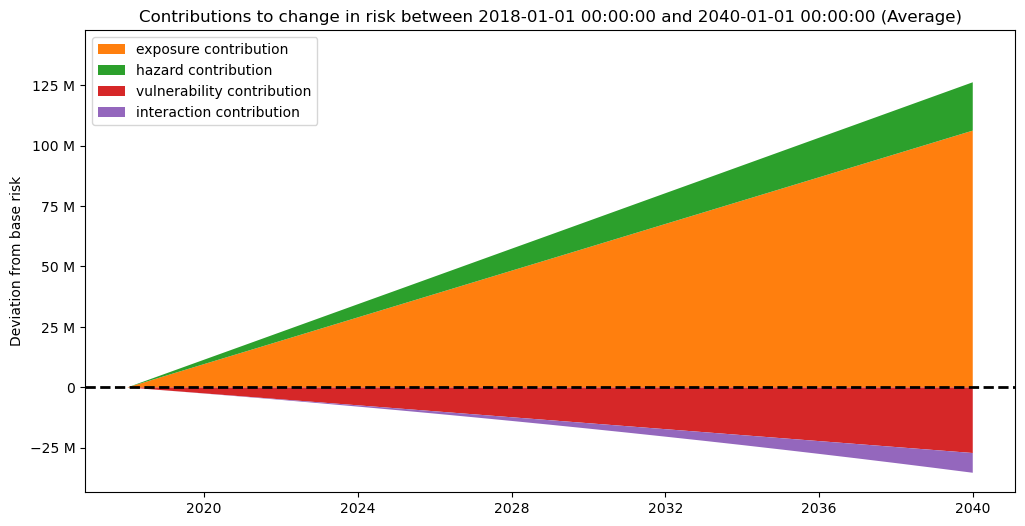
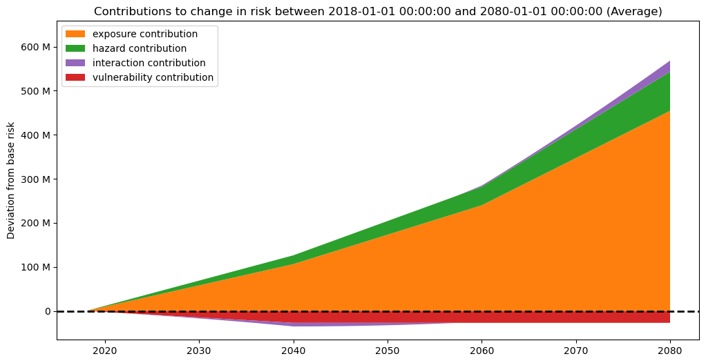
And as well on a per date basis (keep in mind this is an interpolation, thus should be interpreted with caution):

interpolated_risk_traj.plot_time_waterfall()

(<Figure size 1200x600 with 1 Axes>,
 <Axes: title={'center': 'Contributions to change in risk between 2018-01-01 00:00:00 and 2040-01-01 00:00:00 (Average)'}, ylabel='Deviation from base risk'>)

DiscRates

To correctly assess the future risk, you may also want to apply a discount rate, in order to express future costs in net present value.

This can easily be done providing an instance of the already existing DiscRates class when instantiating the trajectory.

The discount rate is applied by assuming the year of the date of the first Snapshot is the baseline (no discounting).

Note that when interpolating on a sub-yearly basis, the discount rate remains on a yearly basis: All dates

from climada.entity import DiscRates
import numpy as np

year_range = np.arange(exp_present.ref_year, exp_future.ref_year + 1)
annual_discount_stern = np.ones(n_years) * 0.014
discount_stern = DiscRates(year_range, annual_discount_stern)
discounted_risk_traj = InterpolatedRiskTrajectory(
    snapcol, risk_disc_rates=discount_stern
)

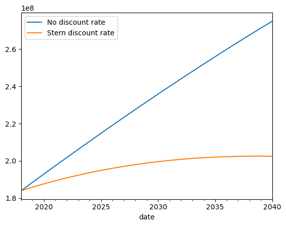
You can easily notice the difference with the previously defined trajectory without discount rate.

ax = interpolated_risk_traj.aai_metrics().plot(
    x="date", y="risk", label="No discount rate"
)
discounted_risk_traj.aai_metrics().plot(
    x="date", y="risk", label="Stern discount rate", ax=ax
)

<Axes: xlabel='date'>

When to use Static vs Interpolated trajectories?

StaticTrajectory objects do not bring new information compared to usual impact computation with ImpactCalc, they are just a way to ease computations and results handling over many different triplets at different dates.

Conversely, InterpolatedTrajectory objects bring an interpolated estimate of risk (per change in risk component), in between the dates. This can be useful when estimates of the risk in between two dates matters, for instance:

• To evaluate when certain thresholds are reached.

• When stress-testing across a time horizon

• To integrate with other related time-series

Advanced usage

In this section we present some more advanced features and use of this module.

Exposure sub groups

It is often useful to look at sub-groups of your exposure (social groups of different social vulnerability, buildings of different type, etc.)

The trajectory module facilitate looking at risk specifically for sub-groups of exposure points. In order to do so, you need to set a column “group_id” in the GeoDataFrame of your exposure.

Here we create dummy groups for exposure points above and below the mean exposure value:

exp_present.gdf["group_id"] = (
    exp_present.gdf["value"] > exp_present.gdf["value"].mean()
) * 1
exp_future.gdf["group_id"] = (
    exp_future.gdf["value"] > exp_future.gdf["value"].mean()
) * 1

snap1 = Snapshot(
    exposure=exp_present, hazard=haz_present, impfset=impf_set, date="2018"
)
snap2 = Snapshot(exposure=exp_future, hazard=haz_future, impfset=impf_set, date="2040")
static_risk_traj = StaticRiskTrajectory([snap1, snap2])
interpolated_risk_traj = InterpolatedRiskTrajectory([snap1, snap2])

You can now access the aii_per_group metric, which will give you the average impact (for the frequency unit of you hazard) restricted to the exposure points of the corresponding group.

static_risk_traj.aai_per_group_metrics()

	date	group	measure	metric	unit	risk
0	2018-01-01	0	no_measure	aai	USD	6.094866e+06
1	2018-01-01	1	no_measure	aai	USD	1.508360e+08
2	2040-01-01	0	no_measure	aai	USD	1.063804e+07
3	2040-01-01	1	no_measure	aai	USD	2.642915e+08

interpolated_risk_traj.aai_per_group_metrics().head()

	date	group	measure	metric	unit	risk
0	2018	0	no_measure	aai	USD	6.094866e+06
1	2018	1	no_measure	aai	USD	1.508360e+08
2	2019	0	no_measure	aai	USD	6.285071e+06
3	2019	1	no_measure	aai	USD	1.555734e+08
4	2020	0	no_measure	aai	USD	6.476829e+06

Results caching

Trajectory objects regroup a large number of computations, especially for the interpolated ones. The module makes use of both a caching process to avoid recomputing the same metric over and over, and a “lazy” flow, which means computations are run only when needed.

As such, the first time you call any metric can take a bit of time, but the subsequent ones should be much faster.

Modifying attributes that would change the results (e.g. the time resolution or the impact computation strategy), will reset the cache.

However this caching process can also get memory expensive. So you can deactivate it by setting “trajectory_caching” to false in CLIMADA’s configuration (see Configuration).

Higher number of snapshots

You can of course use the module to evaluate more that two snapshots. With the StaticRiskTrajectory you will get a collection of results for each snapshot.

For the InterpolatedRiskTrajectory the interpolation will be done between each pair of consecutive snapshots and all results will be collected together, this is usefull if you want to explore a trajectory for which you have clear “intermediate points”, for instance if you are evaluating the risk in an area for which you know some specific development projects will start at a certain date.

Below is an example featuring three snapshots:

from climada.engine.impact_calc import ImpactCalc
from climada.util.api_client import Client
from climada.entity import ImpactFuncSet, ImpfTropCyclone
from climada.trajectories.snapshot import Snapshot
from climada.trajectories import InterpolatedRiskTrajectory
import copy

client = Client()

future_years = [2040, 2060, 2080]

exp_present = client.get_litpop(country="Haiti")
haz_present = client.get_hazard(
    "tropical_cyclone",
    properties={
        "country_name": "Haiti",
        "climate_scenario": "historical",
        "nb_synth_tracks": "10",
    },
)

impf_set = ImpactFuncSet([ImpfTropCyclone.from_emanuel_usa()])
exp_present.gdf.rename(columns={"impf_": "impf_TC"}, inplace=True)
exp_present.gdf["impf_TC"] = 1
exp_present.gdf["group_id"] = (exp_present.gdf["value"] > 500000) * 1

snapcol = [
    Snapshot(exposure=exp_present, hazard=haz_present, impfset=impf_set, date="2018")
]

for year in future_years:
    exp_future = copy.deepcopy(exp_present)
    exp_future.ref_year = year
    n_years = exp_future.ref_year - exp_present.ref_year + 1
    growth_rate = 1.02
    growth = growth_rate**n_years
    exp_future.gdf["value"] = exp_future.gdf["value"] * growth

    haz_future = client.get_hazard(
        "tropical_cyclone",
        properties={
            "country_name": "Haiti",
            "climate_scenario": "rcp60",
            "ref_year": str(year),
            "nb_synth_tracks": "10",
        },
    )
    impf_set = ImpactFuncSet(
        [
            ImpfTropCyclone.from_emanuel_usa(v_half=78.0),
        ]
    )
    exp_future.gdf.rename(columns={"impf_": "impf_TC"}, inplace=True)
    exp_future.gdf["impf_TC"] = 1
    snapcol.append(
        Snapshot(
            exposure=exp_future, hazard=haz_future, impfset=impf_set, date=str(year)
        )
    )

2026-03-27 14:39:45,922 - climada.entity.exposures.base - INFO - Reading /home/sjuhel/climada/data/exposures/litpop/LitPop_150arcsec_HTI/v3/LitPop_150arcsec_HTI.hdf5
2026-03-27 14:39:51,177 - climada.hazard.io - INFO - Reading /home/sjuhel/climada/data/hazard/tropical_cyclone/tropical_cyclone_10synth_tracks_150arcsec_HTI_1980_2020/v2/tropical_cyclone_10synth_tracks_150arcsec_HTI_1980_2020.hdf5
2026-03-27 14:39:56,312 - climada.hazard.io - INFO - Reading /home/sjuhel/climada/data/hazard/tropical_cyclone/tropical_cyclone_10synth_tracks_150arcsec_rcp60_HTI_2040/v2/tropical_cyclone_10synth_tracks_150arcsec_rcp60_HTI_2040.hdf5
2026-03-27 14:40:01,428 - climada.hazard.io - INFO - Reading /home/sjuhel/climada/data/hazard/tropical_cyclone/tropical_cyclone_10synth_tracks_150arcsec_rcp60_HTI_2060/v2/tropical_cyclone_10synth_tracks_150arcsec_rcp60_HTI_2060.hdf5
2026-03-27 14:40:06,967 - climada.hazard.io - INFO - Reading /home/sjuhel/climada/data/hazard/tropical_cyclone/tropical_cyclone_10synth_tracks_150arcsec_rcp60_HTI_2080/v2/tropical_cyclone_10synth_tracks_150arcsec_rcp60_HTI_2080.hdf5

risk_traj = InterpolatedRiskTrajectory(snapcol)

The “static” waterfall plot shows the evolution of risk between the earliest and latest snapshot.

risk_traj.plot_waterfall()

<Axes: title={'center': 'Evolution of the contributions of risk between 2018 and 2080 (Average impact)'}, ylabel='USD'>

risk_traj.plot_time_waterfall()

(<Figure size 1200x600 with 1 Axes>,
 <Axes: title={'center': 'Contributions to change in risk between 2018-01-01 00:00:00 and 2080-01-01 00:00:00 (Average)'}, ylabel='Deviation from base risk'>)

Non-default return periods

You can easily change the default return periods computed, either at initialisation time, or via the property return_periods. Note that estimates of impacts for specific return periods are highly dependant on the data you provided.

We cannot check if the event set you provide is fit for computing impacts for a specific return period.

snapcol = [snap1, snap2]
risk_traj = InterpolatedRiskTrajectory(snapcol, return_periods=[10, 15, 20, 30])
display(risk_traj.return_periods_metrics())

risk_traj.return_periods = [150, 250, 500]
display(risk_traj.return_periods_metrics())

	date	group	measure	metric	unit	risk
0	2018	All	no_measure	rp_10	USD	1.225210e+07
1	2019	All	no_measure	rp_10	USD	1.277500e+07
2	2020	All	no_measure	rp_10	USD	1.330821e+07
3	2021	All	no_measure	rp_10	USD	1.385172e+07
4	2022	All	no_measure	rp_10	USD	1.440553e+07
...	...	...	...	...	...	...
87	2036	All	no_measure	rp_30	USD	8.662373e+08
88	2037	All	no_measure	rp_30	USD	8.894772e+08
89	2038	All	no_measure	rp_30	USD	9.129904e+08
90	2039	All	no_measure	rp_30	USD	9.367770e+08
91	2040	All	no_measure	rp_30	USD	9.608368e+08

92 rows × 6 columns

	date	group	measure	metric	unit	risk
0	2018	All	no_measure	rp_150	USD	8.436864e+09
1	2019	All	no_measure	rp_150	USD	8.697801e+09
2	2020	All	no_measure	rp_150	USD	8.960766e+09
3	2021	All	no_measure	rp_150	USD	9.225760e+09
4	2022	All	no_measure	rp_150	USD	9.492784e+09
...	...	...	...	...	...	...
64	2036	All	no_measure	rp_500	USD	2.643662e+10
65	2037	All	no_measure	rp_500	USD	2.698681e+10
66	2038	All	no_measure	rp_500	USD	2.753977e+10
67	2039	All	no_measure	rp_500	USD	2.809551e+10
68	2040	All	no_measure	rp_500	USD	2.865402e+10

69 rows × 6 columns

Non-yearly date index

You can use any valid pandas frequency string for periods for the time resolution, for instance “5Y” for every five years. This reduces the resolution of the interpolation, which can reduce the required computations at the cost of “precision”. Conversely you can also increase the time resolution to a monthly base for instance.

Same as for the return periods, you can change that at initialisation or afterward via the property.

Keep in mind that risk metrics are still computed the same way, so if you initialy had hazards with annual frequency values, you would still have “Average Annual Impacts” values for every months and not average monthly ones!

Also note that InterpolatedRiskTrajectory uses PeriodIndex for the time dimension. These indexes are defined with the dates of the first and last snapshot, and the given time resolution.

This means that an InterpolatedRiskTrajectory for a 2020 Snapshot and 2040 Snapshot with a yearly time resolution will include all years from 2020 to 2040 included (11 years in total).

However, a trajectory with the same snapshots with a monthly resolution will have January 2040 as a last period if you only provided year 2040 for the last date. If you want to include the whole 2040 year, you need to explicitly give the date “2040-12-31” to the last snapshot.

snapcol = [snap1, snap2]
risk_traj = InterpolatedRiskTrajectory(snapcol, time_resolution="5Y")
risk_traj.per_date_risk_metrics().head()

	date	group	measure	metric	unit	risk
0	2018	All	no_measure	aai	USD	1.569309e+08
1	2023	All	no_measure	aai	USD	1.845465e+08
2	2028	All	no_measure	aai	USD	2.134182e+08
3	2033	All	no_measure	aai	USD	2.435459e+08
4	2038	All	no_measure	aai	USD	2.749295e+08

## snapcol = [snap, snap2]

## Here we use "1MS" to get a monthly basis
risk_traj.time_resolution = "1M"

## We would have to divide results by 12 to get "average monthly impacts"
risk_traj.per_date_risk_metrics()

	date	group	measure	metric	unit	risk
0	2018-01	All	no_measure	aai	USD	1.569309e+08
1	2018-02	All	no_measure	aai	USD	1.573399e+08
2	2018-03	All	no_measure	aai	USD	1.577492e+08
3	2018-04	All	no_measure	aai	USD	1.581589e+08
4	2018-05	All	no_measure	aai	USD	1.585688e+08
...	...	...	...	...	...	...
1585	2039-11	1	no_measure	aai	USD	2.633593e+08
1586	2039-12	0	no_measure	aai	USD	1.061942e+07
1587	2039-12	1	no_measure	aai	USD	2.638252e+08
1588	2040-01	0	no_measure	aai	USD	1.063804e+07
1589	2040-01	1	no_measure	aai	USD	2.642915e+08

1590 rows × 6 columns

Non-linear interpolation

The module allows you to define your own interpolation strategy. Thus you can decide how to interpolate along each dimension of risk (Exposure, Hazard and Vulnerability). This is done via InterpolationStrategy objects, which simply require three functions stating how to interpolate along each dimensions.

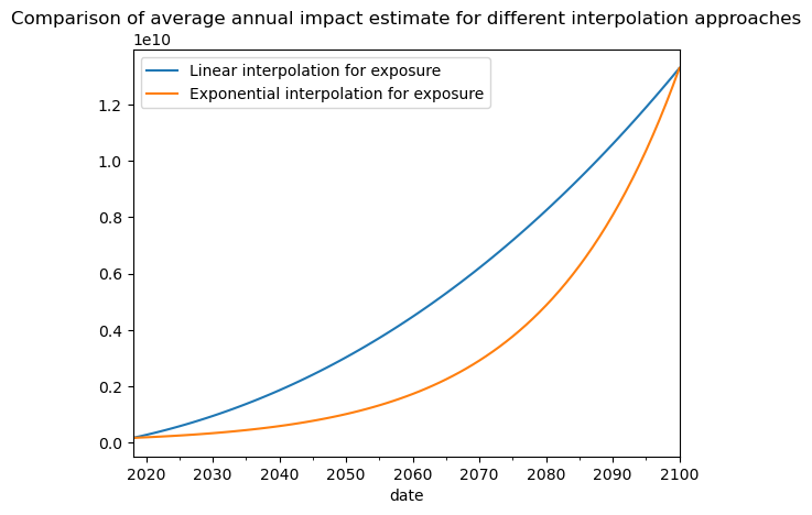
For convenience the module provides an AllLinearStrategy (the risk is linearly interpolated along all dimensions) and a ExponentialExposureStrategy (uses exponential interpolation along exposure, and linear for the two other dimensions).

This can prove helpfull if you are interpolating between two distant dates with an exponential growth factor for the exposure value. On the example below, we show the difference in risk estimates using an the two different interpolation strategies for the exposure dimension:

from climada.trajectories import StaticRiskTrajectory, InterpolatedRiskTrajectory
from climada.trajectories import ExponentialExposureStrategy
import seaborn as sns

future_year = 2100
exp_future = copy.deepcopy(exp_present)
exp_future.ref_year = future_year
n_years = exp_future.ref_year - exp_present.ref_year + 1
growth_rate = 1.04
growth = growth_rate**n_years
exp_future.gdf["value"] = exp_future.gdf["value"] * growth

haz_future = client.get_hazard(
    "tropical_cyclone",
    properties={
        "country_name": "Haiti",
        "climate_scenario": "rcp60",
        "ref_year": "2080",
        "nb_synth_tracks": "10",
    },
)
impf_set = ImpactFuncSet(
    [
        ImpfTropCyclone.from_emanuel_usa(v_half=60.0),
    ]
)
exp_future.gdf.rename(columns={"impf_": "impf_TC"}, inplace=True)
exp_future.gdf["impf_TC"] = 1

snap2 = Snapshot(exposure=exp_future, hazard=haz_future, impfset=impf_set, date="2100")
snapcol = [snap1, snap2]

exp_interp = ExponentialExposureStrategy()
risk_traj = InterpolatedRiskTrajectory(snapcol)
risk_traj_exp = InterpolatedRiskTrajectory(snapcol, interpolation_strategy=exp_interp)
ax = risk_traj.aai_metrics().plot(
    x="date", y="risk", label="Linear interpolation for exposure"
)
risk_traj_exp.aai_metrics().plot(
    x="date", y="risk", label="Exponential interpolation for exposure", ax=ax
)

ax.set_title(
    "Comparison of average annual impact estimate for different interpolation approaches"
)

2026-03-27 14:40:21,528 - climada.hazard.io - INFO - Reading /home/sjuhel/climada/data/hazard/tropical_cyclone/tropical_cyclone_10synth_tracks_150arcsec_rcp60_HTI_2080/v2/tropical_cyclone_10synth_tracks_150arcsec_rcp60_HTI_2080.hdf5

Text(0.5, 1.0, 'Comparison of average annual impact estimate for different interpolation approaches')

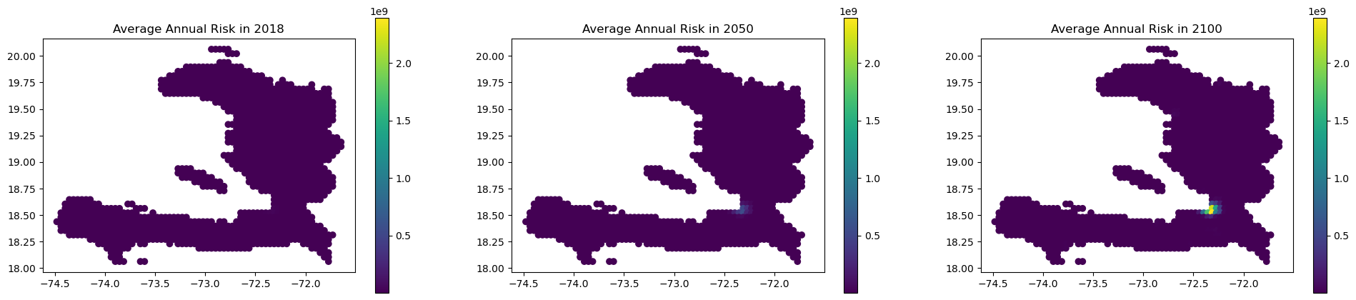
Spatial mapping

You can access a DataFrame with the estimated annual impacts at each coordinates through “eai_metrics” which can easily be merged to the exposure GeoDataFrame:

df = risk_traj.eai_metrics()
df

	date	group	measure	metric	unit	coord_id	risk
0	2018	0	no_measure	eai	USD	0	2993.678321
1	2019	0	no_measure	eai	USD	0	3994.537003
2	2020	0	no_measure	eai	USD	0	5038.235198
3	2021	0	no_measure	eai	USD	0	6125.062545
4	2022	0	no_measure	eai	USD	0	7255.308683
...	...	...	...	...	...	...	...
110302	2096	0	no_measure	eai	USD	1328	99978.314476
110303	2097	0	no_measure	eai	USD	1328	102320.813007
110304	2098	0	no_measure	eai	USD	1328	104694.867359
110305	2099	0	no_measure	eai	USD	1328	107100.640151
110306	2100	0	no_measure	eai	USD	1328	109538.294005

110307 rows × 7 columns

import matplotlib.pyplot as plt

gdf = snap1.exposure.gdf
gdf["coord_id"] = gdf.index
gdf = gdf.merge(df, on="coord_id")

fig, axs = plt.subplots(1, 3, figsize=(24, 5))

gdf.loc[gdf["date"] == "2018-01-01"].plot(
    column="risk",
    legend=True,
    vmin=gdf["risk"].min(),
    vmax=gdf["risk"].max(),
    ax=axs[0],
)
gdf.loc[gdf["date"] == "2050-01-01"].plot(
    column="risk",
    legend=True,
    vmin=gdf["risk"].min(),
    vmax=gdf["risk"].max(),
    ax=axs[1],
)
gdf.loc[gdf["date"] == "2100-01-01"].plot(
    column="risk",
    legend=True,
    vmin=gdf["risk"].min(),
    vmax=gdf["risk"].max(),
    ax=axs[2],
)

axs[0].set_title("Average Annual Risk in 2018")
axs[1].set_title("Average Annual Risk in 2050")
axs[2].set_title("Average Annual Risk in 2100")

plt.show()

Custom Impact Computation strategy

By default, trajectory objects use ImpactCalc().impact() to compute the Impact object and the resulting metric, but you can customize this behaviour via the impact_computation_strategy argument.

The value has to be a class derived from ImpactComputationStrategy, and should at the very least implement a compute_impacts() method, taking Exposures, Hazard and ImpactFuncSet arguments and returning an Impact object.

For instance, if you don’t want the matching of the exposure and hazard centroids to be done internally you can do the following:

from climada.trajectories.impact_calc_strat import ImpactComputationStrategy


class ImpactCalcNoAssign(ImpactComputationStrategy):
    def compute_impacts(
        self,
        exp,
        haz,
        vul,
    ):
        return ImpactCalc(exposures=exp, impfset=vul, hazard=haz).impact(
            assign_centroids=False
        )

Note that you now have to assign the centroids before running the computations or else they will fail:

exp_present = client.get_litpop(country="Haiti")
exp_present.gdf.rename(columns={"impf_": "impf_TC"}, inplace=True)
exp_present.gdf["impf_TC"] = 1


exp_future = copy.deepcopy(exp_present)
exp_future.gdf["value"] = exp_future.gdf["value"] * growth

exp_present.assign_centroids(haz_present)
exp_future.assign_centroids(haz_future)

snap1 = Snapshot(
    exposure=exp_present, hazard=haz_present, impfset=impf_set, date="2018"
)
snap2 = Snapshot(exposure=exp_future, hazard=haz_future, impfset=impf_set, date="2040")

impact_calc_no_assign = ImpactCalcNoAssign()

static_risk_traj = StaticRiskTrajectory(
    [snap1, snap2], impact_computation_strategy=impact_calc_no_assign
)

2026-03-27 14:40:25,488 - climada.entity.exposures.base - INFO - Reading /home/sjuhel/climada/data/exposures/litpop/LitPop_150arcsec_HTI/v3/LitPop_150arcsec_HTI.hdf5
2026-03-27 14:40:25,501 - climada.entity.exposures.base - INFO - Matching 1329 exposures with 1332 centroids.
2026-03-27 14:40:25,504 - climada.util.coordinates - INFO - No exact centroid match found. Reprojecting coordinates to nearest neighbor closer than the threshold = 0.08333333333331439 degree
2026-03-27 14:40:25,508 - climada.entity.exposures.base - INFO - Matching 1329 exposures with 1332 centroids.
2026-03-27 14:40:25,511 - climada.util.coordinates - INFO - No exact centroid match found. Reprojecting coordinates to nearest neighbor closer than the threshold = 0.08333333333331439 degree

static_risk_traj.per_date_risk_metrics()

2026-03-27 14:40:25,564 - climada.trajectories.calc_risk_metrics - WARNING - No group id defined in the Exposures object. Per group aai will be empty.

	date	group	measure	metric	unit	risk
0	2018-01-01	All	no_measure	aai	USD	4.027184e+08
1	2040-01-01	All	no_measure	aai	USD	1.330047e+10
2	2018-01-01	All	no_measure	rp_20	USD	4.096584e+08
3	2040-01-01	All	no_measure	rp_20	USD	2.003911e+10
4	2018-01-01	All	no_measure	rp_50	USD	7.738183e+09
5	2040-01-01	All	no_measure	rp_50	USD	2.719459e+11
6	2018-01-01	All	no_measure	rp_100	USD	1.351303e+10
7	2040-01-01	All	no_measure	rp_100	USD	4.438845e+11